If you have \(X_1,\ldots,X_n\) independent from an \(N(\mu,1)\) distribution you don’t have to think too hard to work out that \(\bar X_n\), the sample mean, is the right estimator of \(\mu\) (unless you have quite detailed prior knowledge). As people who have taken an advanced course in mathematical statistics will know, there is a famous estimator that appears to do better.
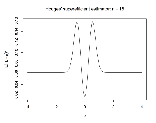
Hodges’ estimator is given by \(H_n=\bar X_n\) if \(|\bar X_n|>n^{-1/4}\), and \(H_n=0\) if \(|\bar X_n|\leq n^{-1/4}\). If \(\mu\neq 0\), \(H_n=\bar X_n\) for all large enough \(n\), so \[\sqrt{n}(H_n-\mu)\stackrel{d}{\to}N(0,1)\] just as for \(\bar X_n\). On the other hand, if \(\mu=0\), \[\sqrt{n}(H_n-\mu)\stackrel{p}{\to}0.\] \(H_n\) is asymptotically better than \(\bar X_n\) for \(\mu=0\) and asymptotically as good for any other value of \(\mu\). Of course there’s something wrong with it: it sucks for \(n^{-1/2}\ll\mu<n^{-1/4}\). Here’s its mean squared error:
Even Wikipedia knows this much. What I recently got around to doing was extending this to an estimator that’s asymptotically superior to \(\bar X_n\) on a dense set. This isn’t new – Le Cam did it in his PhD thesis. It may even be the same as Le Cam’s construction (which isn’t online, as far as I can tell). [Actually, Le Cam’s construction is a draft exercise in a draft chapter for David Pollard’s long-awaited ‘Asymptopia’. And it is basically my one, so it’s quite likely that as a Pollard fan I got at least the idea from there.]
First, instead of just setting the estimate to zero when it’s close enough to zero, we can set it to the nearest integer when it’s close enough to an integer. Define \(\tilde H_n=i\) if \(|\bar X_n-i|<0.5n^{-1/4}\), with \(\tilde H_n=\bar X_n\) otherwise.
If \(n\) is large enough, we can shrink to multiples of 1/2. For example, using the same threshold for closeness, if \(n>16\) there is at most one multiple of 1/2 within \(0.5n^{-1/4}\). If \(n>256\) there is at most one multiple of 1/4 within that range.
Define \(H_{n,k}=2^{-k}i\) if \(|x-2^{-k}i|< 0.5n^{-1/4}\) and \(H_{n,k}=\bar X_n\) otherwise. This is well-defined if \(n>2^{4k}\). For any fixed \(k\), \(\tilde H_{n,k}\) satisfies \[\sqrt{n}(H_n-\mu)\stackrel{p}{\to}0\] if \(\mu\) is a multiple of \(2^{-k}\) and \[\sqrt{n}(H_n-\mu)\stackrel{d}{\to}N(0,1)\] otherwise.
The obvious thing to do now is to let \(k\) increase slowly with \(n\). This doesn’t work. Consider a value for \(\mu\) whose binary expansion has infinitely many 1s, but with increasingly many zeroes between them. Whatever your rule for \(k(n)\) there will be values of this type that are close enough to multiples of \(2^{-k(n)}\) to get pulled to the wrong value infinitely often as \(n\) increases. \(H_{n,k(n)}\) will be asymptotically superior to \(\bar X_n\) on a dense set, but it will be asymptotically inferior on another dense set, violating the rules of the game.
What we can do is pick \(k\) at random. The efficiency gain isn’t 100% as it was for fixed \(k\), but it’s still there.
Let \(K\) be a random variable with probability mass function \(p(k)\), independent of the \(X\)s. The distribution of \(H_{n,K}\) conditional on \(K=k\) is the distribution of \(H_{n,k}\). If \(p(k)>0\) for all \(k\), the probability of seeing \(K=k\) infinitely often is 1, so we can look the limiting distribution of \(\sqrt{n}(H_{n,K}-\mu)\) along subsequences with \(K=k\). This limiting distribution is a point mass at zero if \(2^k\mu\) is an integer, and \(N(0,1)\) otherwise. So, \[\sqrt{n}(H_{n,K}-\mu)\stackrel{d}{\to}q_k\delta_0+(1-q_k)N(0,1)\] where \[q_k=\sum_k p_k I(2^k\mu\textrm{ is an integer})\]
For a dense set of real numbers, and in particular for all numbers representable in binary floating point, \(H_{n,K}\) has greater asymptotic efficiency than the efficient estimator \(\bar X_n.\) The disadvantage of this randomised construction is that working out the finite-sample MSE is just horrible to think about.
The other interesting thing to think about is why the ‘overflow’ heuristic doesn’t work. Why doesn’t superefficiency for all fixed \(k\) translate into superefficiency for sufficiently-slowly increasing \(k(n)\)? As a heuristic, this sort of thing has been around since the early days of analysis, but it’s more than that: the field of non-standard analysis is basically about making it rigorous.
My guess is that \(H_{n,k}\) for infinite \(n\) is close to the superefficient distribution on the dense set only for ‘large enough’ infinite \(k\), and close to \(N(0,1)\) off the dense set only for ‘small enough’ infinite \(k\). The failure of the heuristic is similar to the failure in Cauchy’s invalid proof that a convergent sequence of continuous functinons has a continuous limit, the proof into which later analysis retconned the concepts of ‘uniform convergence’ and ‘equicontinuity’.